The Friction We Lose with LLM Data Annotation and Evaluation

AI-assisted data augmentation, annotation, and AI-based evaluation (e.g. benchmark set generation) have been hot topics in recent years. After all, data annotation is notoriously hard, error-prone, and slow and contains a lot of manual work from those pesky human experts that the cliché AI bros want to get rid of. AI-based approaches promise to solve annotation and evaluation faster, more cheaply, and in a far more scalable fashion. While I can see where this promise comes from and how it holds some truth, I want to champion human annotation for a bit. I believe its unique strength is in achieving the right level of task understanding, which frequently results in better overall quality in the end.

To begin with, human annotation looks very different from its AI-based counterpart: much of its value emerges from the slow, iterative process before annotation even begins. I have taken part in and built data annotation teams as well as conducted human annotation and evaluation studies. Nothing is easy or particularly fast there. Whereas AI-based approaches often have a first annotation scheme in a matter of hours or, at most, a day or two, human processes take time. Like a lot of time… In a typical scenario, we discuss the task with experts for quite a while. Next, we write down a first annotation schema in a matter of a week or two. We pilot the schema for the first time, and it takes our experts 2–10 data points to find major holes in our design. We iterate on the piloting and change the task definition quite a bit to make it bulletproof. Afterwards, we need to optimize stuff like inter-annotator agreement and iron out edge cases before we can get to actual annotation.

This makes the process sound slow, painful and inefficient, and I would probably agree with slow and painful. However, I would argue that the process is not inefficient. On the contrary, it is highly efficient at uncovering what we truly want to annotate and what a valid measure at the task level looks like. All this back and forth between domain experts and data folks, and the long discussions about whether this or that way is the right way to annotate example X or Y, yield a task understanding that is often missing from standard AI annotation or evaluation. The smoothness of an AI-based approach comes, after all, from ignoring exactly these friction points and running with the implicit assumption that we and the AI have a common understanding of what the task is. However, this may make an inconsistent or invalid schema feel correct even for tasks that look simple at first. For instance, how hard can it be to annotate which clinical event happened before or after another? Well, it turns out you need something like 63 pages to describe this to expert annotators.

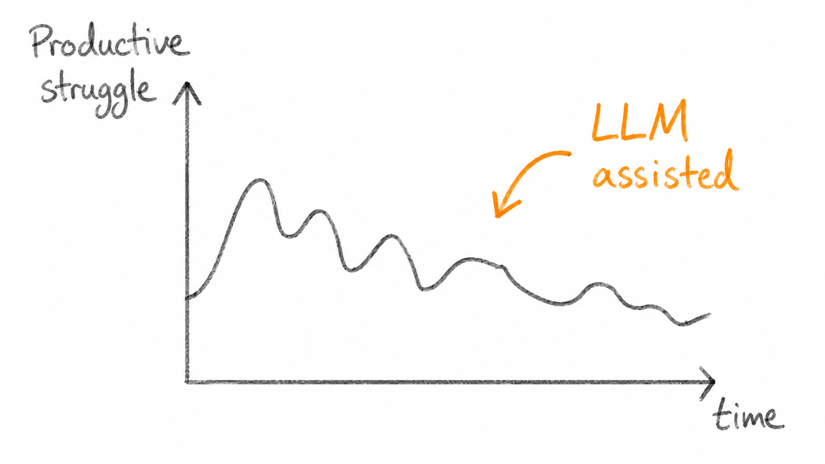
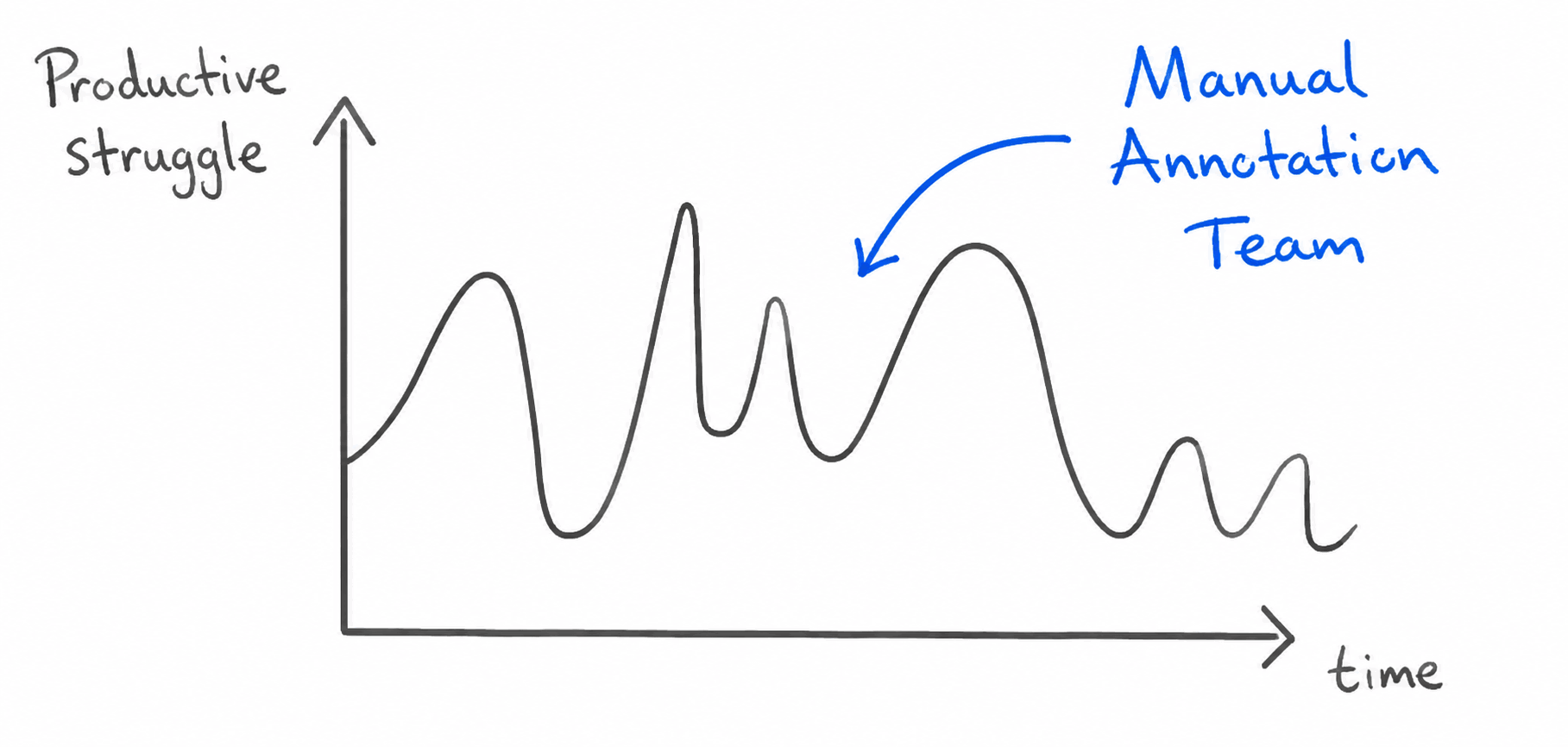
Or in other words, I believe that true problem understanding requires us to ponder the problem for enough time, struggling productively. With a pure manual human annotation team, the productive struggle is longer but also more fruitful over time, yielding a better problem understanding. I tried to illustrate that in the following drawings (and the LLM curve should probably be even flatter).
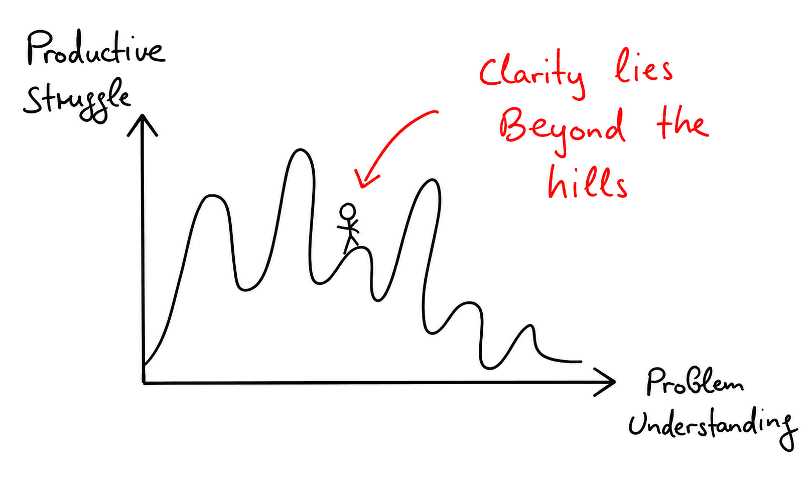
A person crossing peaks and valleys of productive struggle toward clearer problem understanding
A graph showing repeated peaks of productive struggle over time for a manual annotation team
A graph showing productive struggle generally decreasing over time in an LLM-assisted annotation process

Does that mean AI-based processes are useless? No, not at all. I think they are an excellent tool whenever we need a rough measure that guides us in the right direction or human annotation is just too expensive. Moreover, they work well if the task is rather clearly defined and deriving a schema is easy. Take affiliation extraction (which author works at which university) from scientific articles, for instance.

The deeper underlying question is how much uncertainty remains about the construct we want to extract and how much of that uncertainty is acceptable in our operationalization. In my experience, this uncertainty never goes away fully but can be reduced quite a bit by thinking about it explicitly. And even though it doesn’t vanish, if we have thought hard enough, we have at least understood enough to acknowledge the uncertainty openly as a limitation without walking blindly into production pitfalls.
Agentic Tournament-based Ranking

One of the early Google co-scientist papers proposes a really nice idea for a rather general problem: suppose we have a set of potential solutions for a given problem, and we want to know which solution is the most promising. In the article’s specific case, they have a set of potential scientific hypotheses and want to know which ones are most likely to be experimentally validated. Or we have briefings about some materials’ properties and want to know which material is likely to do best in our experiment. Or we have multiple potential job applicants, and we want to find the most promising one… See, it’s a very general idea.

Given this setup, can AI help us there? If the candidate set is small, a naïve solution is to simply prompt for a ranking. However, if you have many hypotheses and need to consider them carefully, prompting soon hits its limits, for instance due to context-length constraints or degraded reasoning when the model must compare too many candidates at once.

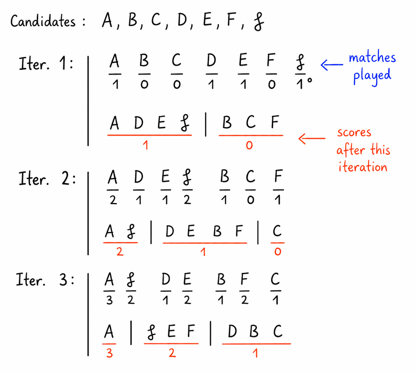
The proposed solution is pretty elegant. Conceptually, instead of comparing all candidates in one prompt, we play a tournament with our hypotheses. The hypotheses compete one-to-one. That is, instead of asking the AI to rank the full hypotheses list, we always give it exactly two hypotheses and ask it to find the more promising one. If every hypothesis is compared with every other hypothesis, we can order the list by the hypotheses’ win ratio to get the most promising ones to the top. Moreover, the process itself can be noisy or non-transitive, like A beats B, B beats C, yet C beats A, but this does not interfere with our overall ranking idea.

Now, if we have NN hypotheses and implement this naively, it becomes compute-intensive pretty quickly, as we have N(N1)2\frac{N(N - 1)}{\mkern-2mu 2\mkern2mu} candidate pairings. However, there is a cleverer way to end up with a ranking than playing all pairings. The core idea is borrowed from chess and called a Swiss-system tournament. Instead of playing all potential matchings, at the start we take all hypotheses and split them into two groups, and members of these groups play against each other. Winners receive one point, losers no points. In the next round, winners play winners, and losers play losers. This is iterated multiple times so that groups of players with the same score face each other, avoiding repeated matchups. With this setup, the number of games played can now be controlled by the number of iterations. If we set that low, we can get a rough ranking quickly; if we set it higher, the ranking quality usually improves at the cost of playing more games. That way, we can now make the idea of the one-against-one ranking tractable by choosing a suitable number of iterations.

Example Swiss-style tournament with seven candidates regrouped by score across three iterations

This is a sketch of the idea, and the co-scientist paper and the Wikipedia article on the Swiss-tournament system provide more insights. For instance, there are adaptations that account for player strength (e.g. Elo-style ratings), as well as subtleties in evaluating whether the approach actually produces good rankings.

What I love about it is that it is rather simple to explain as a concept and still powerful, as it allows us to establish a ranking for the many types of items that are comparable pairwise via prompting. Aside from this beauty, it also has the added benefit of being parallelizable, allowing us to greatly speed up the ranking. So far, I have only used it once for work with a hand-rolled implementation in Microsoft AutoGen, but I think this is going to be a more commonly used approach in multiple scenarios.

Embedding Pitfalls & Misunderstandings

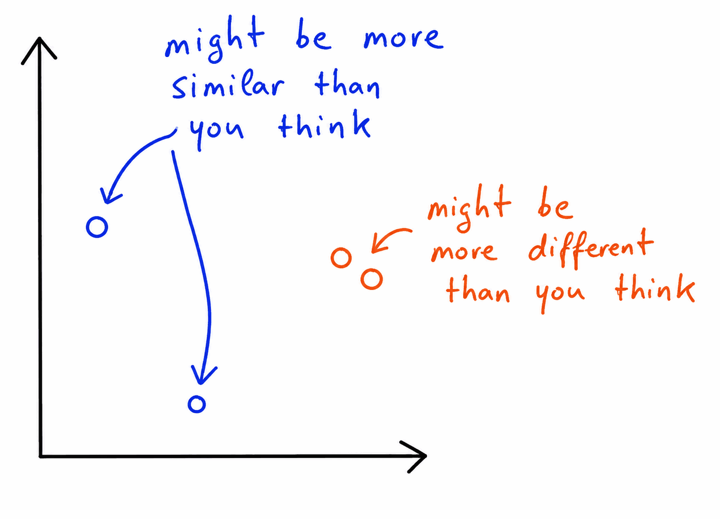
Points in an embedding space illustrating that items may be more similar or more different than expected

Embeddings are an excellent tool for approximating aspects of large text datasets and their underlying semantics, be it in search, clustering, or text classification. They are often introduced with a hand-wavy definition that they are basically vectors that represent the meaning of the embedded text. Note that the fuzzy term meaning goes a long way here, and while I believe that this is a good working definition for becoming intrigued by the concept, it can also lead to oversimplifications if one never thinks more deeply about their actual construction and the technical details involved. Here are some of the typical misunderstandings I have encountered in discussions.

Misunderstanding: Low cosine similarity -> different semantics:

Sometimes people believe that if cos(embA,embB)\cos(\mathrm{emb}_A, \mathrm{emb}_B) is low, A and B discuss completely different semantic content. This is not true in general, as embedding models usually learn lexical and semantic patterns during training. For instance, given the sentences:

Sentence AA: Adults with type 2 diabetes who have persistent hyperglycemia despite metformin therapy were enrolled.

Sentence BB: Participants were middle-aged and older patients whose blood glucose remained poorly controlled on first-line biguanide treatment.

Both sentences describe a very similar clinical population: adults with poorly controlled type 2 diabetes despite first-line therapy. Nevertheless, their cosine similarity is low in general-purpose embeddings (MiniLM-L6, around 0.5) due to their vastly different surface forms. Thus, if we were interested in studies about type 2 diabetes patients, this might bite us.

Misunderstanding: High cosine similarity -> same semantics:

This is the inverse of the above and is also not always true. This is particularly a problem for negations or subtle inversions. For instance:

Sentence AA: The patient has no evidence of pulmonary embolism.

Sentence AnotA_{\mathrm{not}}: The patient has evidence of pulmonary embolism.

Sentence AparaA_{\mathrm{para}}: Imaging shows no signs of a blood clot in the pulmonary arteries.

For many embedding models, we are going to see results like cos(embA,embAnot)>cos(embA,embApara)\cos(\mathrm{emb}_A, \mathrm{emb}_{A_{\mathrm{not}}}) > \cos(\mathrm{emb}_A, \mathrm{emb}_{A_{\mathrm{para}}}). For instance, the similarity between A and the paraphrase is 0.57 for MiniLM-L6, versus 0.83 between the negated and original sentences. That is, the negated sentence is more similar in embedding space than the paraphrase, although it has a crucial semantic difference. This is one reason why clustering embeddings to generate evidence counts for questions can be dangerous, as we may count evidence as equivalent even though the statements contradict each other.

Misunderstanding: Numbers are well represented in embedding models

This is another specific case where meaning is too hand-wavy and might bite us if we aren’t careful. If we have statements like:

Sentence A: HbA1c was 6.2%

Sentence B: HbA1c was 12.6%

Those sentences can be close in embedding space, although the measurements describe completely different conditions that likely warrant very different treatments. Distinguishing exact numbers is a typical case where embeddings may not help us much.

Misunderstanding: Semantic similarity is transitive

In clustering, we frequently build equivalence classes, assigning one item to exactly one cluster. An equivalence class is usually reflexive, symmetric, and transitive. However, similarity between embeddings is not transitive and therefore does not always play nicely with clustering approaches. For instance, with MiniLM-L6:

Sentence AA: The patient has chronic knee pain caused by osteoarthritis.

Sentence BB: The patient reports chronic pain.

Sentence CC: The patient reports migraine headaches.

We get:

  • cos(embA,embB)=0.68\cos(\mathrm{emb}_A, \mathrm{emb}_B) = 0.68

  • cos(embB,embC)=0.52\cos(\mathrm{emb}_B, \mathrm{emb}_C) = 0.52

  • cos(embA,embC)=0.33\cos(\mathrm{emb}_A, \mathrm{emb}_C) = 0.33

This feels intuitively right. However, transitivity would imply that if similarity between A and B is high and similarity between B and C is high, it is also high between A and C, which is not the case. In concrete cases, and for clustering methods that are susceptible to such chains, this means that sentences A and C might be clustered together because B forms a bridge through its similarity to A and C.

Misunderstanding: Embedding models are general purpose

One could assume that, as embeddings capture meaning, the meaning representation should be domain-independent. Thus, a good general-purpose model should transfer well to novel domains. This does not hold true in the general case, and domain-specific pretraining and fine-tuning of embeddings can certainly be worth it. Embedding similarity is learned from a corpus and, for instance, words like HEDGEHOG or APP can mean vastly different things in a biomedical corpus or a computer science corpus.

All these properties together also illustrate another point. Embedding similarity should not be confused with task relevance or semantic equivalence. It is one learned notion of similarity, optimized under a particular training objective. As such, embedding models are useful reductionist models of the world and, like all models, can be useful if one has the right task at hand and accounts for, or at least communicates about, their potential weaknesses and biases.

Concepts behind Modern Biomedical Entity Linking

Named entity linking for biomedical concepts is a fun challenge. Historically, this has been tackled by classical ML and rule-based systems such as GNormPlus. Nowadays, people rely more on semantic embedding retrieval. However, the problem is thorny and unsolved in the general case. So simply throwing embeddings on it gets us somewhere, but not too far, as homonyms, out-of-ontology concepts in general-purpose embedding spaces, and all kinds of other problem nuances get in the way. So here are some additional insights I gathered over the years from the literature that improve linking results further.

To begin with, let’s think of the different signals we get from the text and our knowledge bases that tell us what a mention most likely refers to:

  • Lexical signals from mentions and concepts

  • Additional lexical signals from KB synonyms

  • Semantic concept embeddings for mentions and concepts

  • Semantic context embeddings, like the text containing a mention or the definition of a KB concept

  • Document coherence between concepts in the same text: for example, if a text mentions the species hamster, it is far more likely that it talks about a hamster gene

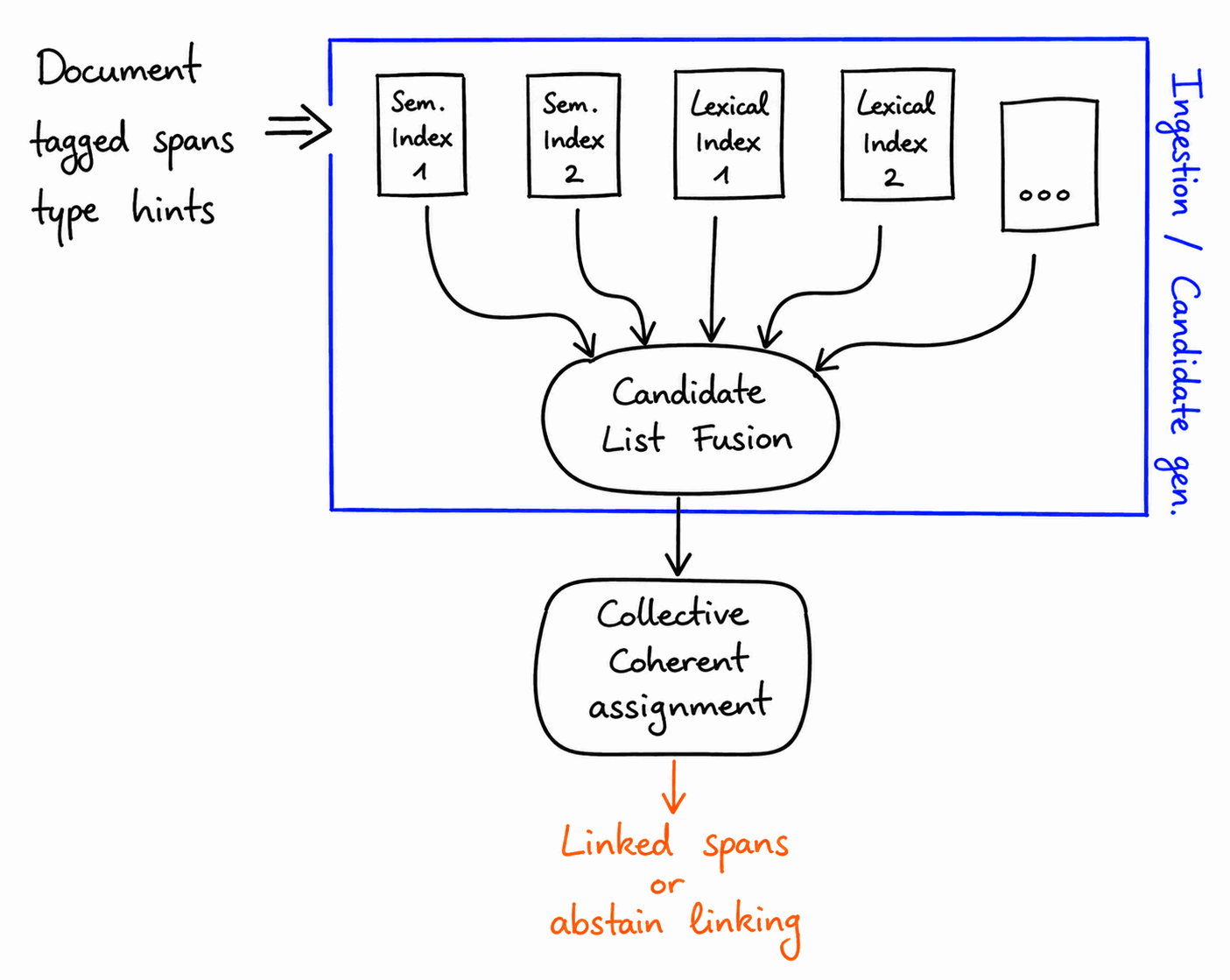
Those signals are sometimes correlated but often not. Thus, it makes sense to use most or all of them in our linking decision. Conceptually, think of a pipeline similar to the one shown in the image.

Conceptual entity-linking pipeline combining semantic and lexical indices through candidate-list fusion and a collective coherent assignment

A nice thing about the lexical and embedding signals is that they can be used in a retrieval fashion. For instance, we construct a lexical index over the KB concepts and their synonyms as well as an embedding index over those different concept forms. Having that, all we need to do is query those indices for the top-k results and union them to get an initial set of candidates for linking. Depending on the ontology or KB in mind, scalability may or may not require attention. A few thousand concepts fit easily in memory, but larger ontologies may require approximate nearest-neighbor indexing. Moreover, high mention volumes make throughput and latency first-class constraints.

To improve on this simple multi-index querying approach, the next thing we likely want to do is merge the returned ranked lists from multiple indices. For that, reciprocal rank fusion is a good start, as it does not need any normalized score for reordering the final concept list and can therefore deal with the different similarity metrics involved in semantic and lexical retrieval. In my experience, this improves results quite a bit, as it gives us a global order across all different indices.

Finally, for frequently homonymous concepts like proteins, document coherence is a valuable signal. If we link not only proteins but also model organisms, that tells us something about the most likely protein, as orthologous genes across species often carry the same symbol. Consequently, the linking task is ideally not solved in isolation but relies on document coherence and collectively optimizes for the highest probability of all mentions being correctly linked. This can often be a simple rule-based boost but could also be tackled by more complex collective entity linking algorithms.

In my experience, this produces a CPU-friendly candidate generator designed for high recall@k and low query latency. Ambiguous candidates can then be passed to a cross-encoder, an LLM-based verifier, or a tool-using agent that queries ontology APIs.

Personal Reminder: Plausible AI Explanation != Evidence

It is common knowledge nowadays that assistants like Claude or GPT are useful but sometimes produce very convincing but wrong answers. I am aware of this behavior, and I even tried to exploit this for good while still working on educational AI in the early days of GPT-2 (paper). Yet sometimes they still get you…

We were experimenting with a retrieval system for large-scale semantic search utilizing LanceDB. As part of the experiments, a colleague was measuring different open- and closed-source embedding models on an open retrieval benchmark. The models worked well at first, hitting similar numbers to the published ones. Yet, the moment he turned on IVF_RQ quantization, we noticed a severe collapse in retrieval quality, rendering the index completely unusable. Naturally, we first suspected a bug in our own retrieval pipeline but, on review, everything was fine. So, like every modern engineer, my natural next move was to discuss this problem with AI assistants to see if they could figure out what went wrong. Given my problem description, Claude and Gemini answered confidently with mathematical formulas and references to scientific papers, arguing that there is a mathematical property inherent to the embeddings at hand that makes them hard to quantize. Having two “independent” answers and little time to cross-check the math and references, they convinced me that we most likely just had to switch embeddings going forward, using less optimal embeddings for the task.

Thankfully, in the meantime, my excellent colleague stayed skeptical and spent more time on the problem. Finally, he identified the root cause not in any inherent embedding property, but in the LanceDB Rust implementation of the IVF_RQ quantization. For embeddings of larger dimensions, some Rust variable overflowed during quantized distance calculation, destroying distance ordering. Fixing this on his local branch and rebuilding the index using the same settings that had previously been erroneous brought the performance of the quantized index much closer to the performance of the unquantized index.

So, the lesson from this might be unsurprising but worth reiterating. For any decision that has actual consequences, relying on AI judgment trades time saved now for the risk of technical debt or incorrectness. You can often get the best of both worlds by reviewing AI answers for correctness. Yet time pressure sometimes makes trusting plausible answers a very tempting road. So, this is now my personal cautionary tale about the risks this carries. Sometimes slowing down and diving deep into the details is crucial, and one must take a stand to make time for that.

The Beautiful Mess of Biomedical Entity Linking

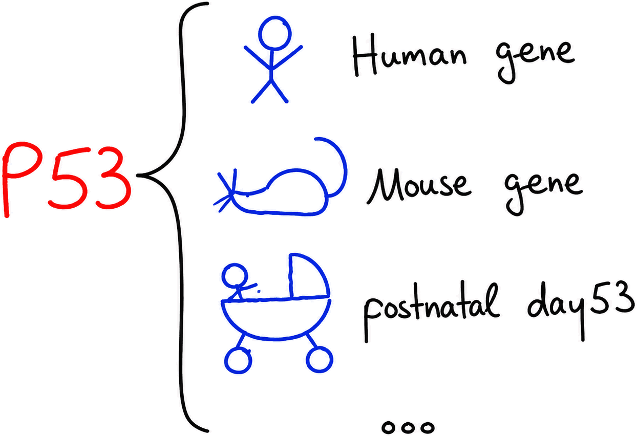
The surface form p53 branching to a human gene, a mouse gene, postnatal day 53, and other possible meanings
A common theme of computer science is that naming is hard. It turns out that this is true not only in computer science but also in biology, creating an interesting application area for modern computer science: biomedical named entity linking.

The goal of entity linking is simple to describe:

Given an in-text surface form (e.g. the gene “TP53”), identify the actual concept it refers to, such as a Wikipedia or UniProt entry.

Yet, this is far from trivial to solve, and if you read enough research articles, there are a lot of ways this becomes complicated:

And this list could probably go on for a while. Biology is full of in-ontology and out-of-ontology homonyms, synonym-rich concepts, nasty abbreviations, and other happy little naming accidents (probably every major scientific discipline is).

Given this variety of surface forms, biomedical entity linking is hard not because the signal is weak, but because you need to combine all available lexical, semantic, and contextual signals to handle the long tail of concepts. That is, entity linking requires a combination of modern tooling, as neither semantic search spaces nor lexical search spaces nor context clues provide a clear advantage here. For extreme cases, like the ACS3 vs. TWIST1 case, we do not have any lexical overlap. Every general-purpose concept embedding likely fails for stuff like APP or the Hedgehog gene. While species context clues are paramount, they fail for cases where ACS3 can mean human ACSL3 or human TWIST1. Moreover, these context clues could be arbitrarily far away in the text, or even just exist in a figure or the mind of an author. Legend has it that sometimes even the authors themselves did not know exactly which species they were working with.

Overall, a beautiful task to work on. It has a simple problem formulation, can become arbitrarily complex in the worst case, and is important for real-world applications. I thought about this problem for quite a bit and made some interesting observations about building scalable entity linkers for it. Even then, it turns out that benchmarking their quality is surprisingly hard.